Searching for the SS Central America
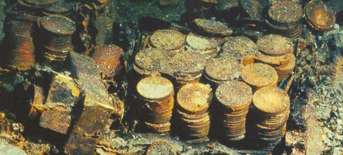
On Tuesday, September 8th 1857, the steamboat SS Central America left Havana at 9 AM for New York, carrying about 600 passengers and crew members. Inside of this vessel, there was stowed a very precious cargo: a set of manuscripts by John James Audubon, and three tons of gold bars and coins. The manuscripts documented an expedition through the yet uncharted southwestern United States and California, and contained 200 sketches and paintings of its wildlife. The gold, fruit of many years of prospecting and mining during the California Gold Rush, was meant to start anew the lives of many of the passengers aboard.
On the 9th, the vessel ran into a storm which developed into a hurricane. The steamboat endured four hard days at sea, and by Saturday morning the ship was doomed. The captain arranged to have women and children taken off to the brig Marine, which offered them assistance at about noon. In spite of the efforts of the remaining crew and passengers to save the ship, the inevitable happened at about 8 PM that same day. The wreck claimed the lives of 425 men, and carried the valuable cargo to the bottom of the sea.
It was not until late 1980s that technology allowed recovery of shipwrecks at deep sea. But no technology would be of any help without an accurate location of the site. In the following paragraphs we would like to illustrate the power of the scipy stack by performing a simple simulation, that ultimately creates a dataset of possible locations for the wreck of the SS Central America, and mines the data to attempt to pinpoint the most probable target.
We simulate several possible paths of the steamboat (say 10,000 randomly generated possibilities), between 7:00 AM on Saturday, and 13 hours later, at 8:00 pm on Sunday. At 7:00 AM on that Saturday the ship’s captain, William Herndon, took a celestial fix and verbally relayed the position to the schooner El Dorado. The fix was 31º25’ North, 77º10’ West. Because the ship was not operative at that point—no engine, no sails—, for the next thirteen hours its course was solely subjected to the effect of ocean current and winds. With enough information, it is possible to model the drift and leeway on different possible paths.
We start by creating a data frame—a computational structure that will hold all the values we need in a very efficient way. We do so with the help of the pandas libraries.
1
2
3
4
5
6
7
8
9
10
11
12
from datetime import datetime, timedelta
from dateutil.parser import parse
import numpy as np, pandas as pd

interval = [parse("9/12/1857 7 am")]
for k in range(14*2-1):
    if k % 2 == 0:
        interval.append(interval[-1])
    else:
        interval.append(interval[-1] + timedelta(hours=1))

herndon = pd.DataFrame(np.zeros((28, 10000)), index = [interval, ['Lat', 'Lon']*14])
Each column of the data frame herndon is to hold the latitude and longitude of a possible path of the SS Central America, sampled every hour. Let us populate this data following a similar analysis to the one followed by the Columbus America Discovery Group, as explained by Lawrence D. Stone in the article Revisiting the SS Central America Search, from the 2010 Conference on Information Fusion.
The celestial fix obtained by Capt. Herndon at 7:00 AM was taken with a sextant in the middle of a storm. There are some uncertainties in the estimation of latitude and longitude with this method and under those weather conditions, which are modeled by a bivariate normally distributed random variable with mean (0,0) and standard deviations of 0.9 nautical miles (for latitude), and 3.9 nautical miles (for longitude). We create first a random variable with those characteristics. Let us use this idea to populate the dataframe with several random initial locations.
1
2
from scipy.stats import multivariate_normal
celestial_fix = multivariate_normal(cov = np.diag((0.9, 3.9)))
To estimate the corresponding celestial fixes, as well as all further geodetic computations, we will use the accurate formulas of Vincenty for ellipsoids, assuming a radius at the Equator of \(a = 63781374\) meters, and a flattening of the ellipsoid of \(f = 1/298.257223563\) (these figures are regarded as one of the standards for use in cartography, geodesy and navigation, and are referred by the community as the World Geodetic System WGS-84 ellipsoid)
A very good set of Vincenty’s formulas coded in python can be found at wegener.mechanik.tu-darmstadt.de/GMT-Help/Archiv/att-8710/Geodetic_py.
In particular, for this example we will be using Vincenty’s direct formula, that computes the resulting latitude \(\phi_2\), longitude \(\lambda_2\), and azimuth \(\alpha_2\) of an object starting at latitude \(\phi_1\), longitude \(\lambda_1\), and traveling \(s\) meters with initial azimuth \(\alpha_1\). Latitudes, longitudes and azimuths are given in degrees, and distances in meters. We also use the convention of assigning negative values to the latitudes to the West. To apply the conversion from nautical miles or knots to their respective units in SI, we employ the system of units in scipy.constants.
1
2
3
4
5
6
7
8
9
10
from Geodetic_py import vinc_pt
from scipy.constants import nautical_mile
a = 6378137.0
f = 1./298.257223563
for k in range(10000):
    lat_delta, lon_delta = celestial_fix.rvs() * nautical_mile
    azimuth = 90 - np.angle(lat_delta + 1j*lon_delta, deg=True)
    distance = np.hypot(lat_delta, lon_delta)
    output = vinc_pt(f, a, 31+25./60, -77-10./60, azimuth, distance)
    herndon.ix['1857-09-12 07:00:00',:][k] = output[0:2]
Issuing now the command herndon.ix['1857-09-12 07:00:00',:] gives us the following output:
--------------------------------------------------------------------------------
          0          1          2          3          4          5     \
Lat  31.455345  31.452572  31.439491  31.444000  31.462029  31.406287
Lon -77.148860 -77.168941 -77.173416 -77.163484 -77.169911 -77.168462
          6          7          8          9       ...           9990  \
Lat  31.390807  31.420929  31.441248  31.367623    ...      31.405862
Lon -77.178367 -77.187680 -77.176924 -77.172941    ...     -77.146794
          9991       9992       9993       9994       9995       9996  \
Lat  31.394365  31.428827  31.415392  31.443225  31.350158  31.392087
Lon -77.179720 -77.182885 -77.159965 -77.186102 -77.183292 -77.168586
          9997       9998       9999
Lat  31.443154  31.438852  31.401723
Lon -77.169504 -77.151137 -77.134298
[2 rows x 10000 columns]
--------------------------------------------------------------------------------
We simulate the drift according to the formula \(D = (V + \gamma W)\). In this formula \(V\) (the ocean current) is modeled as vector pointing about North-East (around 45 degrees of azimuth) and a variable speed between 1 and 1.5 knots. The other random variable, \(W\), represents the action of the winds in the area during the hurricane, which we choose to represent by directions ranging between South and East, and speeds with a mean 0.2 knots, standard deviation 1/30 knots. Both random variables are coded as bivariate normal. Finally, we have accounted for the leeway factor. According to a study performed on the blueprints of the SS Central America, we have estimated this leeway \(\gamma\) to be about 3%.
This choice of random variables to represent the ocean current and wind differs from the ones used in the aforementioned paper. In our version we have not used the actual covariance matrices as computed by Stone from data received from the Naval Oceanographic Data Center. Rather, we have presented a very simplified version.
1
2
3
4
5
6
7
8
9
10
11
12
13
14
15
current = multivariate_normal((np.pi/4, 1.25), cov=np.diag((np.pi/270, .25/3)))
wind    = multivariate_normal((np.pi/4, .3), cov=np.diag((np.pi/12, 1./30)))
leeway  = 3./100
for date in pd.date_range('1857-9-12 08:00:00', periods=13, freq='1h'):
    before  = herndon.ix[date-timedelta(hours=1)]
    for k in range(10000):
        angle, speed = current.rvs()
        current_v = speed * nautical_mile * (np.cos(angle) + 1j * np.sin(angle))
        angle, speed  = wind.rvs()
        wind_v = speed * nautical_mile * (np.cos(angle) + 1j*np.sin(angle))
        drift = current_v + leeway * wind_v
        azimuth = 90 - np.angle(drift, deg=True)
        distance = abs(drift)
        output = vinc_pt(f, a, before.ix['Lat'][k], before.ix['Lon'][k], azimuth, distance)
        herndon.ix[date,:][k] = output[:2]
Let us plot the first three of those simulated paths:
1
2
3
4
5
6
7
8
9
10
11
12
13
14
15
16
import matplotlib.pyplot as plt
from mpl_toolkits.basemap import Basemap
m = Basemap(llcrnrlon=-77.4, llcrnrlat=31.2, urcrnrlon=-76.6,
            urcrnrlat=31.8, projection='lcc', lat_0 = 31.5,
            lon_0=-77, resolution='l', area_thresh=1000.)
m.drawmeridians(np.arange(-77.4,-76.6,0.1), labels=[0,0,1,1])
m.drawparallels(np.arange(31.2,32.8,0.1), labels=[1,1,0,0])
colors = ['r', 'b', 'k']
styles = ['-', '--', ':']
for k in range(3):
    longitudes = herndon[k][:,'Lon'].values
    latitudes  = herndon[k][:,'Lat'].values
    longitudes, latitudes = m(longitudes, latitudes)
    m.plot(longitudes, latitudes, color=colors[k], lw=3, ls=styles[k])

plt.show()
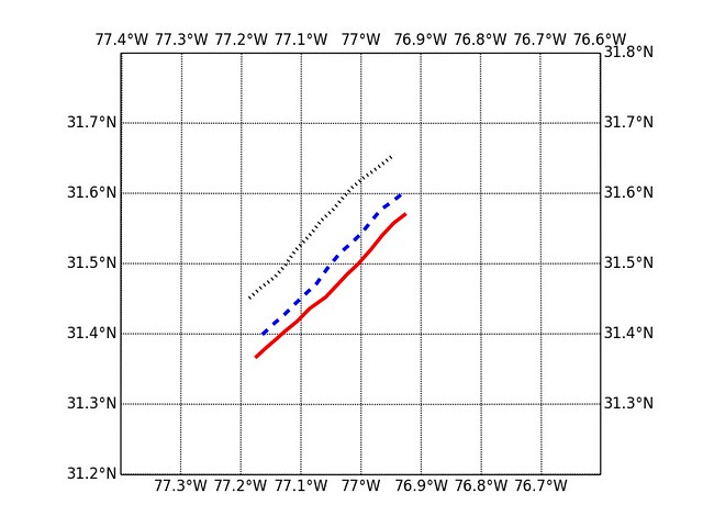
As expected they observe a North-Easterly general direction, in occasion showing deviations from the effect of the strong winds.
The advantage of storing all the different steps in these paths becomes apparent if we need to perform some further study—and maybe filtering—on the data obtained. We could impose additional conditions to paths, and use only those filtered according to the extra rules, for example. Another advantage is the possibility of performing different analysis on the paths with very little coding. By issuing the command herndon.loc(axis=0)[:,'Lat'].describe(), we obtain quick statistics on the computed latitudes for all 10000 paths (number of items, mean, standard deviation, min, max and the quartiles of the data).
--------------------------------------------------------------------------------
0 1 2 3 4 5 \
count 14.000000 14.000000 14.000000 14.000000 14.000000 14.000000
mean 31.474706 31.489831 31.479797 31.551953 31.543533 31.516511
std 0.058218 0.060026 0.060504 0.060204 0.060290 0.065008
min 31.388410 31.400693 31.387974 31.457087 31.446786 31.421331
25% 31.431773 31.439437 31.429712 31.506764 31.498132 31.465424
50% 31.470768 31.491100 31.481918 31.551521 31.546649 31.510613
75% 31.515063 31.541353 31.527317 31.599800 31.588251 31.568368
max 31.571535 31.580176 31.575999 31.641745 31.639944 31.619281
6 7 8 9 ... 9990 \
count 14.000000 14.000000 14.000000 14.000000 ... 14.000000
mean 31.463063 31.515181 31.510682 31.448281 ... 31.541765
std 0.064530 0.060904 0.064621 0.061350 ... 0.059633
min 31.369973 31.410879 31.412623 31.353806 ... 31.445757
25% 31.410827 31.473212 31.460292 31.398931 ... 31.500659
50% 31.460968 31.516328 31.511749 31.448647 ... 31.542774
75% 31.512171 31.565814 31.555854 31.492793 ... 31.583822
max 31.564134 31.601316 31.620487 31.547686 ... 31.632320
9991 9992 9993 9994 9995 9996 \
count 14.000000 14.000000 14.000000 14.000000 14.000000 14.000000
mean 31.481608 31.501862 31.509630 31.495412 31.557487 31.491508
std 0.064426 0.061343 0.057857 0.068578 0.058520 0.055164
min 31.384021 31.398002 31.408542 31.387861 31.452803 31.402979
25% 31.422987 31.457732 31.468419 31.440465 31.518770 31.450746
50% 31.489742 31.509546 31.515301 31.503460 31.565790 31.493993
75% 31.532992 31.549224 31.553803 31.545975 31.596499 31.532340
max 31.576120 31.589048 31.591815 31.599973 31.645622 31.577492
9997 9998 9999
count 14.000000 14.000000 14.000000
mean 31.522756 31.509904 31.461305
std 0.055411 0.064045 0.066058
min 31.435634 31.408430 31.363115
25% 31.482015 31.458449 31.405953
50% 31.523253 31.519991 31.463235
75% 31.567399 31.555133 31.516251
max 31.605647 31.605175 31.556127
[8 rows x 10000 columns]
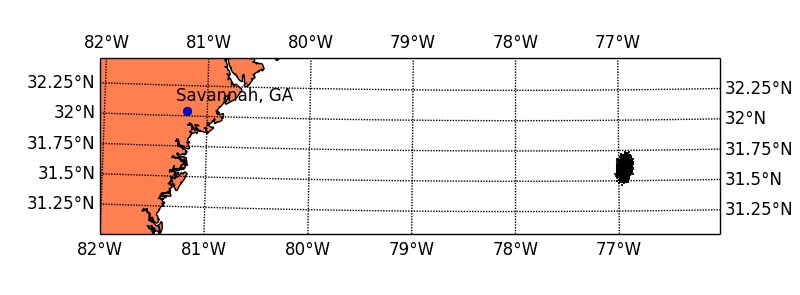
--------------------------------------------------------------------------------The focus of this simulation is, nonetheless, on the final location of all these paths. Let us plot them all on the same map first, for a quick visual evaluation.
1
2
3
4
5
6
7
8
9
10
11
12
13
14
15
16
latitudes, longitudes = herndon.ix['1857-9-12 20:00:00'].values
m = Basemap(llcrnrlon=-82., llcrnrlat=31, urcrnrlon=-76,
            urcrnrlat=32.5, projection='lcc', lat_0 = 31.5,
            lon_0=-78, resolution='h', area_thresh=1000.)
longitudes, latitudes = m(longitudes, latitudes)
x, y = m(-81.2003759, 32.0405369)  # Coordinates of Savannah, GA
m.plot(longitudes, latitudes, 'ko', markersize=1)
m.plot(x,y,'bo')
plt.text(x-10000, y+10000, 'Savannah, GA')
m.drawmeridians(np.arange(-82,-76,1), labels=[1,1,1,1])
m.drawparallels(np.arange(31,32.5,0.25), labels=[1,1,0,0])
m.drawcoastlines()
m.drawcountries()
m.fillcontinents(color='coral')
m.drawmapboundary()
plt.show()