Interaction with Sage
The objective of this post is to show a few examples of interaction of sage with \( \LaTeX \) to produce results that, otherwise, would carry extensive writing and computation on the side. We will base it on the figure from the post Sequence of Right Triangles, where right triangles were constructed by halving one of their angles, placing one of the legs on the hypotenuse of the previous triangle, and point the second leg towards the \( x \)–axis.
In the first example, we show how to get the most of your skills manipulating strings to produce a sage script that generates a tikz code. In the second example, we utilize the full power of the graphing capabilities of sage to accomplish a similar result.
The mathematical background is nonetheless the same for both examples: According to the results shown in the relevant post, we need to concern only with the position of the vertices at the end of the hypotenuses: We can think of those as vectors \( v_n \) that can be expressed in polar coordinates by \( \theta=\tfrac{\pi}{2^n}, \rho=2^n \sin\big( \tfrac{\pi}{2^{n+1}} \big). \)
Interaction of sage with tikz
We are looking for a string of characters that codes the construction of the triangles in tikz language: A possible quick sage script that would generate such a string holding up to \( n \) triangles in this fashion, could be something like this:
1
2
3
4
5
6
7
8
9
10
m = 1
n = 5
output = ""
while (m <=n):
    m=m+1
    s = pi/2^(m+1)
    h = 2^m*sin(pi/2^(m+1))
    smo = pi/2^m
    hmo = 2^(m-1)*sin(pi/2^m)
    output += r"\draw (0cm,0cm)--(%f r:%fcm)--(%f r:%fcm)--cycle;"%(s,h,smo,hmo)
Note that, since I chose a while environment, I initialize the counter m=1 outside, an empty string output and for this particular example, chose five steps (n=5). The following four variable declarations simply compute the value of angle (s, smo) and length (h, hmo) of the vectors \( v_m \) and \( v_{m-1} \) respectively, for values of m from 2 to 5. Finally, on each step I append to output the corresponding tikz code that produces the desired triangle.
To insert this code in a \( \LaTeX \) document, all we have to do is wrap it in a sagesilent environment (or sageblock if you want it displayed), and call \sagestr{output} inside of a tikzpicture environment. Something like this:
1
2
3
4
5
6
7
8
9
10
11
12
13
14
15
16
17
18
19
20
21
22
\begin{sagesilent}
m=1
n=5
output=""
while (m <=n):
    m=m+1
    s=pi/2^(m+1)
    h=2^m*sin(pi/2^(m+1))
    smo=pi/2^m
    hmo=2^(m-1)*sin(pi/2^m)
    output+=r"\draw (0cm,0cm)--(%f r:%fcm)--(%f r:%fcm)--cycle;"%(s,h,smo,hmo)
\end{sagesilent}

\begin{center}
\begin{tikzpicture}[scale=2]
\draw[domain=0.001:3.141,smooth,variable=\t,very thick,blue] %
      plot ({\t r}:1.570796*{sin(\t r)}/\t);
\draw[ultra thick,->] (-0.5cm,0cm) -- (2cm,0cm);
\draw[ultra thick,->] (0cm,-0.5cm) -- (0cm,1.5cm);
\draw (0,0) -- (1cm,1cm) -- (0cm,1cm) -- cycle;
\sagestr{output}
\end{tikzpicture}

To make style changes, like adding your own color scheme, filling the triangles with texture, or labeling each vertex, all you need to modify in the code is the tikz bit in the declaration of output+=[...]. In order to produce a different number of triangles, simply change the declaration n=5 to any other value.
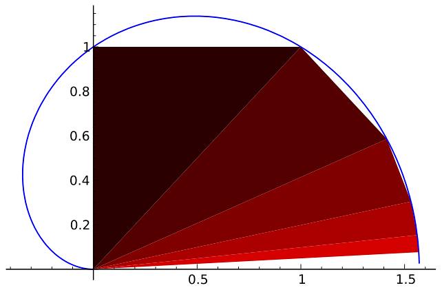
Making the most of the graphing capabilities of sage
It is a no-brainer: we have so much more control over the technical details from within sage, that we can leave the task of rendering and computation directly, to focus on the writing alone. A quick \( \LaTeX \) script that produces a similar result, could look like this:
\begin{sagesilent}
t=polar_plot(pi/2*sin(x)/x,(x,0,pi),color="blue")
for m in range(6):
    s=pi/2^(m+1)
    h=2^m*sin(pi/2^(m+1))
    smo=pi/2^m
    hmo=2^(m-1)*sin(pi/2^m)
    v1=[h*cos(s),h*sin(s)]
    v2=[hmo*cos(smo),hmo*sin(smo)]
    t+=polygon2d([[0,0],v1,v2],rgbcolor=(m/6,0,0))
\end{sagesilent}

\sageplot{t}
As before, we place the actual code that constructs the different plots inside of a sagesilent environment. This code simply creates a polar plot of the required function \( f(\theta) = \tfrac{\sin \theta}{\theta} \) between the angular values of zero and \( \pi \), and then append to it all the triangles, one at a time, by calling the polygon2d command. We take the liberty to change the shade of the triangle inside. That is all. Once the code is finished, we simply call the resulting plot (that was stored in the variable t) with the command \sageplot. Easy, right?