Some results related to the Feuerbach Point

Given a triangle \( \triangle ABC \), the circle that goes through the midpoints of each side, \( D, E, F \), is called the Feuerbach circle. It has very surprising properties:

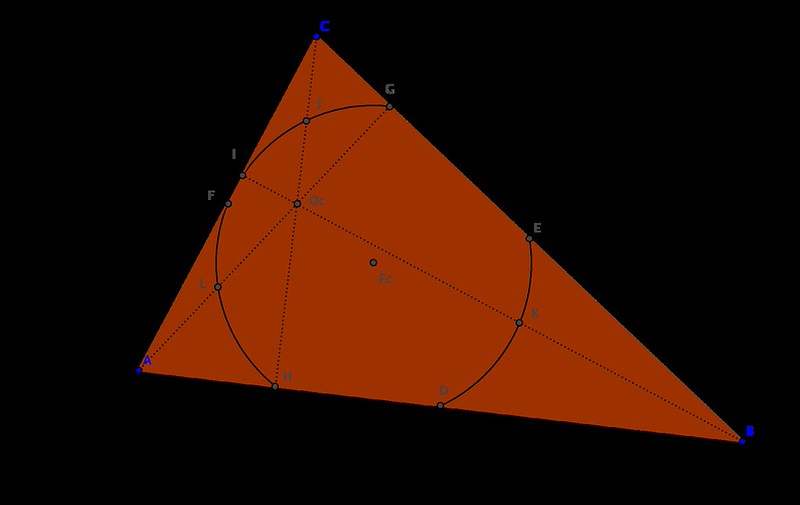
It also goes through the feet of the heights, points \( G, H, I. \)
If \( Oc \) denotes the orthocenter of the triangle, then the Feuerbach circle also goes through the midpoints of the segments \( OcA, OcB, OcC. \) For this reason, the Feuerbach circle is also called the nine-point circle.
The center of the Feuerbach circle is the midpoint between the orthocenter and circumcenter of the triangle.
The area of the circumcircle is precisely four times the area of the Feuerbach circle.

Most of these results are easily shown with sympy without the need to resort to Gröbner bases or Ritt-Wu techniques. As usual, we realize that the properties are independent of rotation, translation or dilation, and so we may assume that the vertices of the triangle are \( A=(0,0), B=(1,0) \) and \( C=(r,s) \) for some positive parameters \( r,s>0. \) To prove the last statement, for instance we may issue the following:

1
2
3
4
5
6
7
8
9
10
11
12
import sympy
from sympy import *

A = Point(0,0)
B = Point(1,0)
r,s = var('r,s')
C = Point(r,s)
D = Segment(A,B).midpoint
E = Segment(B,C).midpoint
F = Segment(A,C).midpoint

simplify(Triangle(A,B,C).circumcircle.area/Triangle(D,E,F).circumcircle.area)

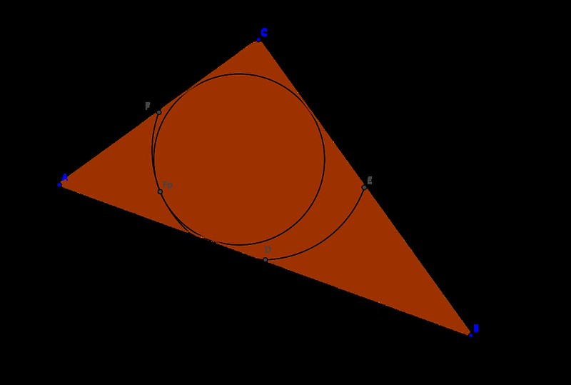
But probably the most amazing property of the nine-point circle, is the fact that it is tangent to the incircle of the triangle. With exception of the case of equilateral triangles, both circles intersect only at one point: the so-called Feuerbach point.

The two results that we want to prove, whose synthetic proofs can be read in [this article] are the following:

Theorem 1. The circle through the feet of the internal bisectors of triangle \( \triangle ABC \) passes through the Feuerbach point of the triangle.

Theorem 2. The Feuerbach point of triangle \( \triangle ABC \) is the anti-Steiner point of the Euler line of the intouch triangle of \( \triangle ABC \) with respect to the same triangle.

Let us prove the first Theorem for the case of a right-triangle. We only need to modify the definition of the point \( C \) to guarantee this situation. We set \( C=(0,s) \) for some positive value of the parameter \( s \).

Let us start by collecting the hypothesis polynomials that define the coordinates \( (x_1,y_1) \) of the Feuerbach point of the triangle \( \triangle ABC. \)

1
2
3
4
5
6
7
import sympy
from sympy import *
A = Point(0,0)
B = Point(1,0)
var('s',positive=True)
C = Point(0,s)
Triangle(A,B,C).incircle.equation()

-s**2/(s + sqrt(s**2 + 1) + 1)**2 + (-s/(s + sqrt(s**2 + 1) + 1) + x)**2
+ (-s/(s + sqrt(s**2 + 1) + 1) + y)**2

We shall introduce the parameter \( u \) in our polynomial rings, and relate it to the parameter \( s \) so that \( u=\sqrt{s^2+1}. \) This will allow us to input the incenter, incircle and their interaction with other objects, in a simple polynomial way.

1
2
3
var('u')
expr = Triangle(A,B,C).incircle.equation().subs(sqrt(s**2+1), u)
numer(together(expr))

-s**2 + (-s + x*(s + u + 1))**2 + (-s + y*(s + u + 1))**2

1
2
3
T = Triangle( Segment(A,B).midpoint, Segment(A,C).midpoint, Segment(B,C).midpoint)
expr = together(T.circumcircle.equation())
numer(expr)

-s**2 + (-s + 4*y)**2 + (4*x - 1)**2 - 1

We can then use the following three polynomials to define the Feuerbach point:

\begin{align} h_1(s,u) &= s^2+1-u^2 \\ h_2(s,u,x_1,y_1) &= (4y-s)^2+(4x-1)^2-1-s^2 \\ h_3(s,u,x_1,y_1) &= \big( (s+u+1)x-s\big)^2+\big((s+u+1)y-s\big)^2-s^2 \\ \end{align}

Let us now proceed to computing the three feet of the internal bisectors, starting by collecting the coordinates of the incenter:

1
2
3
4
5
Ic=Triangle(A,B,C).incenter.subs(sqrt(s**2+1), u)

intersection(Line(A, C), Line(B, Ic))
intersection(Line(A, B), Line(C, Ic))
intersection(Line(B, C), Line(A, Ic))

[Point(0, s/(u + 1))]
[Point(s/(s + u), 0)]
[Point(s/(s + 1), s/(s + 1))]

This gives us the hypothesis polynomials for the coordinates \( (x_2,y_2), (x_3,y_3), (x_4,y_4) \) of the three feet:

\begin{align} h_4(s,u,y_2) &= (u+1)y_2-s \\ h_5(s,u,x_3) &= (s+u)x_3-s \\ h_6(s,u,x_4) &= (s+1)x_4-s \\ h_7(s,u,y_4) &= (s+1)y_4-s \\ \end{align}

Note we do not need to include polynomials for \( x_2 \) or \( y_3 \) since those are always zero. We proceed to compute a polynomial equation of a circle that goes through the last three points:

1
2
3
4
5
6
7
8
var('x2:5 y2:5')

Q1 = Point(0, y2)
Q2 = Point(x3, 0)
Q3 = Point(x4, y4)

expr = together(Triangle(Q1, Q2, Q3).circumcircle.equation())
numer(expr)

-(y2*(-x3**2 + x4**2 + y4**2) + y4*(x3**2 - y2**2))**2 + (2*x*(x3*y4 - y2*(x3 - x4))
- y2*(-x3**2 + x4**2 + y4**2) - y4*(x3**2 - y2**2))**2 + (-x3*(-x3**2 + x4**2 + y4**2)
+ 2*y*(x3*y4 - y2*(x3 - x4)) - (x3 - x4)*(x3**2 - y2**2))**2
- (x3*(-x3**2 + x4**2 + y4**2) - 2*y2*(x3*y4 - y2*(x3 - x4))
+ (x3 - x4)*(x3**2 - y2**2))**2

We thus have the thesis polynomial for the coordinates \( (x_1,y_1) \) of the Feuerbach point to belong on the required circumcircle:

\begin{align} g(s,x_1,y_1,y_2,x_3,x_4,y_4) &= -\left(y_{2} \left(- x_{3}^{2} + x_{4}^{2} + y_{4}^{2}\right) + y_{4} \left(x_{3}^{2} - y_{2}^{2}\right)\right)^{2} \\ & + \left(2 x_1 \left(x_{3} y_{4} - y_{2} \left(x_{3} - x_{4}\right)\right) - y_{2} \left(- x_{3}^{2} + x_{4}^{2} + y_{4}^{2}\right) - y_{4} \left(x_{3}^{2} - y_{2}^{2}\right)\right)^{2} \\ & + \left(- x_{3} \left(- x_{3}^{2} + x_{4}^{2} + y_{4}^{2}\right) + 2 y_1 \left(x_{3} y_{4} - y_{2} \left(x_{3} - x_{4}\right)\right) - \left(x_{3} - x_{4}\right) \left(x_{3}^{2} - y_{2}^{2}\right)\right)^{2} \\ & - \left(x_{3} \left(- x_{3}^{2} + x_{4}^{2} + y_{4}^{2}\right) - 2 y_{2} \left(x_{3} y_{4} - y_{2} \left(x_{3} - x_{4}\right)\right) + \left(x_{3} - x_{4}\right) \left(x_{3}^{2} - y_{2}^{2}\right)\right)^{2} \end{align}

We could use then the following code in sage or sympy in a python session, to prove the result:

1
2
3
4
5
6
7
8
9
10
11
12
13
14
15
16
17
18
19
20
21
22
23
24
25
26
27
28
29
30
31
32
33
34
35
36
37
import sympy
from sympy import var, prem

var('s u x1:5 y1:5)

# Hypotheses for the Feuerbach point
h1 = s**2 + 1 - u**2
h2 = -s**2 + (-s + 4*y1)**2 + (4*x1 - 1)**2 - 1
h3 = -s**2 + (-s + x1*(s + u + 1))**2 + (-s + y1*(s + u + 1))**2

# Hypotheses for the three feet
h4 = (u + 1)*y2 - s
h5 = (s + u)*x3 - s
h6 = (s + 1)*x4 - s
h7 = (s + 1)*y4 - s

# Thesis polynomial
g = -(y2*(-x3**2 + x4**2 + y4**2) + y4*(x3**2 - y2**2))**2 + (2*x1*(x3*y4 - y2*(x3 - x4))
- y2*(-x3**2 + x4**2 + y4**2) - y4*(x3**2 - y2**2))**2 + (-x3*(-x3**2 + x4**2 + y4**2)
+ 2*y1*(x3*y4 - y2*(x3 - x4)) - (x3 - x4)*(x3**2 - y2**2))**2
- (x3*(-x3**2 + x4**2 + y4**2) - 2*y2*(x3*y4 - y2*(x3 - x4))
+ (x3 - x4)*(x3**2 - y2**2))**2

# The system is almost triangular, except for polynomials h2 and h3.
# Substitute those two by the proper pseudo-reminders wrt y1
h3a = prem(h3, h2, y1)
h2a = prem(h2, h3a, y1)

# The proof (by the Ritt-Wu method):
# If the Theorem is true, the last reminder must be zero.
R = prem(g, h7, y4)
R = prem(R, h6, x4)
R = prem(R, h5, x3)
R = prem(R, h4, y2)
R = prem(R, h3a, y1)
R = prem(R, h2a, x1)
R = prem(R, h1)

To prove the second theorem, we need to go over the notion of anti-Steiner points first, and some of their properties:

It is known that there is a one-to-one correspondence between any point in the circumcircle of a triangle \( \triangle ABC \) with a unique line that goes through the orthocenter, via reflections with the sides of the triangle:

If \( P \) is a point belonging to the circumcircle, then the images \( P’,P’‘,P’’’ \) through reflections with axes the three sides of the triangle are collinear, and the corresponding line goes through the orthocenter. This is called the Steiner line of the point \( P. \)
Similarly, if a line \( m \) goes through the orthocenter, then the three reflected lines with the sides of the triangle, \( m’, m’’, m’’’, \) are concurrent at a point of the circumcircle. This is called the anti-Steiner point of the line \( m. \)

It is relatively easy to prove these two facts with sympy (for the geometric computations) and sagemath (for the Gröbner bases calculations). For example, for the first property, we could do as follows: Start by defining a function that computes the reflection of a point with respect to a line.

1
2
3
def reflection(Pt,ln):
	Q = intersection(ln.perpendicular_line(Pt), ln)[0]
	return Point(2*Q.x + Pt.x, 2*Q.y + Pt.y)

Given a generic point \( P=(x,y) \), the three reflections with respect to the sides of the triangle read as follows:

1
2
3
reflection(P, Line(A, B))
reflection(P, Line(B, C))
reflection(P, Line(A, C))

Point(x, -y)
Point(-x + 2*(s**2 + (r - 1)*(r*x + s*y - x))/(s**2 + (r - 1)**2),
	  2*s*(r*x - r + s*y - x + 1)/(s**2 + (r - 1)**2) - y)
Point(2*r*(r*x + s*y)/(r**2 + s**2) - x, 2*s*(r*x + s*y)/(r**2 + s**2) - y)

If the point \( P \) is to belong in the circumcircle of triangle \( \triangle ABC, \) then it must satisfy the corresponding polynomial equation:

1
numer(together(Triangle(A,B,C).circumcircle.equation()))

s**2*(2*x - 1)**2 - s**2 - (r**2 - r + s**2)**2 + (-r**2 + r - s**2 + 2*s*y)**2

This is the (only needed) hypothesis polynomial. The thesis polynomial, that inquires whether the three reflection points are collinear, can be reduced to asking whether the triangle \( \triangle P’P’‘P’’’ \) has area zero:

1
numer(together(Triangle(P1,P2,P3).area))

2*s**2*(r**2*y - r*y + s**2*y - s*x**2 + s*x - s*y**2)

A quick sagemath session proves the result true:

sage: R.<x,y,z,r,s> = PolynomialRing(QQ, 5, order='lex')
sage: h = s**2*(2*x - 1)**2-s**2-(r**2-r+s**2)**2+(-r**2+r-s**2+2*s*y)**2
sage: g = 2*s**2*(r**2*y-r*y+s**2*y-s*x**2+s*x-s*y**2)
sage: I = R.ideal(1-z*g, h)
sage: I.groebner_basis()

[1]