Image Processing with numpy, scipy and matplotlibs in sage

In this post, I would like to show how to use a few different features of numpy, scipy and matplotlibs to accomplish a few basic image processing tasks: some trivial image manipulation, segmentation, obtaining of structural information, etc. An excellent way to show a good set of these techniques is by working through a complex project. In this case, I have chosen the following:

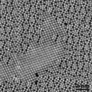
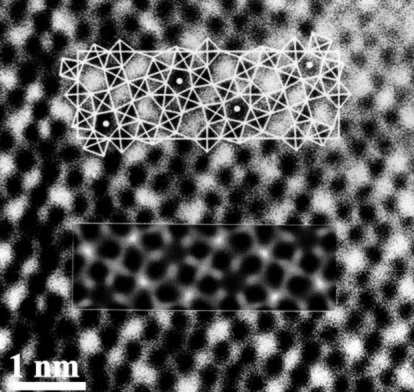
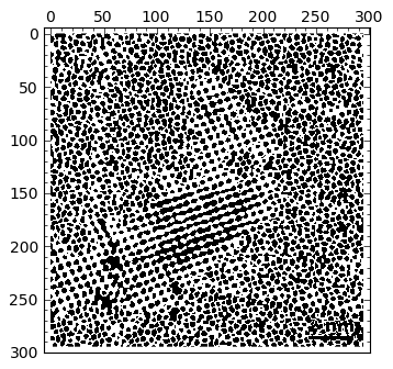
Given a HAADF-STEM micrograph of a bronze-type Niobium Tungsten oxide \( Nb_4W_{13}O_{47} \) (left), find a script that constructs a good approximation to its structural model (right).


Courtesy of ETH Zurich

For pedagogical purposes, I took the following approach to solving this problem:

Segmentation of the atoms by thresholding and morphological operations.
Connected component labeling to extract each single atom for posterior examination.
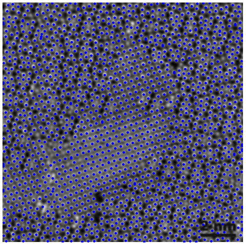
Computation of the centers of mass of each label identified as an atom. This presents us with a lattice of points in the plane that shows a first insight in the structural model of the oxide.
Computation of Delaunay triangulation and Voronoi diagram of the previous lattice of points. The combination of information from these two graphs will lead us to a decent (approximation to the actual) structural model of our sample.

Let us proceed in this direction:

Needed libraries and packages

Once retrieved, our HAADF-STEM images will be stored as big matrices with float32 precission. We will be doing some heavy computations on them, so it makes sense to use the numpy and scipy libraries. From the first module we will retrieve all the functions; from the second, it is enough to retrieve the tools in the scipy.ndimage package (multi-dimensional image processing). The procedures that load those images into matrices, as well as some really good tools to manipulate plots and present them are in the matplotlib libraries; more concretely, matplotlib.image and matplotlib.pyplot. We will use them too. The preamble then looks like this:

1
2
3
4
from numpy import *
import scipy.ndimage
import matplotlib.image
import matplotlib.pyplot

Loading the image

The image is loaded with the command matplotlib.imread(filename). It stores the image as a numpy.ndarray with dtype=float32. Notice that the maxima and minima are respectively 1.0 and 0.0. Other interesting information about the image can be retrieved:

1
2
3
4
5
6
7
8
img = matplotlib.image.imread('/Users/blanco/Desktop/NbW-STEM.png')

print "Image dtype: %s"%(img.dtype)
print "Image size: %6d"%(img.size)
print "Image shape: %3dx%3d"%(img.shape[0], img.shape[1])
print "Max value %1.2f at pixel %6d"%(img.max(), img.argmax())
print "Min value %1.2f at pixel %6d"%(img.min(), img.argmin())
print "Variance: %1.5f\nStandard deviation: %1.5f"%(img.var(), img.std())

Image dtype: float32
Image size:  87025
Image shape: 295x295
Max value 1.00 at pixel  75440
Min value 0.00 at pixel   5703
Variance: 0.02580
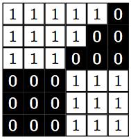
Standard deviation: 0.16062

Thresholding is done, as in matlab, by imposing an inequality on the matrix holding the data. The output is a True-False matrix of ones and zeros, where a one (white) indicates that the inequality is fulfilled, and zero (black) otherwise.


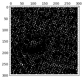`img > 0.2`	`img > 0.7`

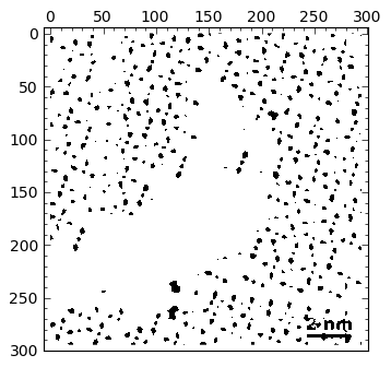
`multiply(img < 0.5,img > 0.25)`	`multiply(img, img > 0.62)`

By visual inspection of several different thresholds, I chose 0.62 as one that gives me a good map showing what I need for segmentation. I need to get rid of “outliers”, though: small particles that might fulfill the given threshold, but are small enough not to be considered an actual atom. Therefore, in the next step I perform a morphological operation of opening to get rid of those small particles: I decided than anything smaller than a quare of size \( 2 \times 2 \) is to be eliminated from the output of thresholding:

1
2
BWatoms = (img  >  0.62)
BWatoms = scipy.ndimage.binary_opening(BWatoms, structure=ones((2,2)))

And we are now ready for segmentation. We perform this task with the scipy.ndimage.label function: It collects one slice per segmented atom, and the number of slices computed. We need to indicate what kind of connectivity is allowed. For example, in the toy example below, do we consider this as one or two atoms?

It all depends: I’d rather have it now as two different connected components, but for some other problems I might consider that they are just one. The way we code it, is by imposing a structuring element that defines feature connections. For example, if our criteria for connectivity between two pixels is that they are in adjacent edges, then the structuring element looks like the image in the left below. If our criteria for connectivity between two pixels is that they are also allowed to share a corner, then the structuring element looks like the image in the right below. For each pixel we impose the chosen structuring element, and count the intersection: if there are no intersections, then the two pixels are not connected. Otherwise, they belong to the same connected component.

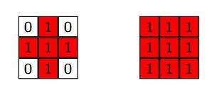
I want to make sure that atoms that are too close in a diagonal direction are counted as two, rather than one, so I chose the structuring element on the left. The script reads then as follows:

1
2
structuring_element = [[0,1,0],[1,1,1],[0,1,0]]
segmentation, segments = scipy.ndimage.label(BWatoms, structuring_element)

Generation of the lattice of the oxide

The object segmentation contains a list of slices, each of them with a True-False matrix containing each of the found atoms of the oxide. We can obtain for each slice a great deal of useful information. For example, the coordinates of the centers of mass of each atom can be retrieved by

1
2
3
coords = scipy.ndimage.center_of_mass(img, segmentation, range(1, segments + 1))
xcoords = array([x[1] for x in coords])
ycoords = array([x[0] for x in coords])

Note that, because of the way matrices are stored in memory, there is a trasposition of the \( x \) and \( y \)-coordinates of the locations of the pixels. No big deal, but we need to take it into account.

Other useful bits of information available:

1
2
3
4
5
6
7
8
9
10
#Calculate the minima and maxima of the values of an array
#at labels, along with their positions.
allExtrema = scipy.ndimage.extrema(img, segmentation, range(1, segments + 1))
allminima = allExtrema[0]
allmaxima = allExtrema[1]
allminimaLocations = allExtrema[2]
allmaximaLocations = allExtrema[3]

# Calculate the mean of the values of an array at labels.
allMeans = scipy.ndimage.means(img, segmentation, range(1, segments + 1))

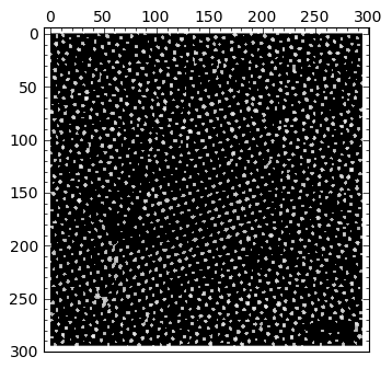
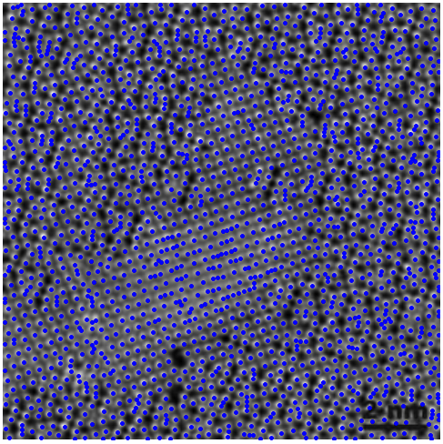
Notice the overlap of the computed lattice of points over the original image (below, left): we have successfully found the centers of mass of most atoms, although there are still about a dozen regions where we are not too satisfied with the result. It is time to fine-tune by the simple method of changing the values of some variables: play with the threshold, with the structuring element, with different morphological operations, etc. We can even add all the obtained information for a wide range of those variables, and filter out outliers. An example with optimized segmentation is shown below (right):

Structural Model of the sample

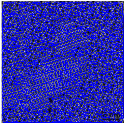
For the purposes of this post, we will be happy providing the Voronoi diagram and Delaunay triangulation of the previous lattice of points. With matplotlib we can take care of the latter with a simple command:

1
triang = matplotlib.tri.Triangulation(xcoords,ycoords)

To show the results, I overlaid the original image (with a forced gray colormap) with the triangulation generated above (in blue).

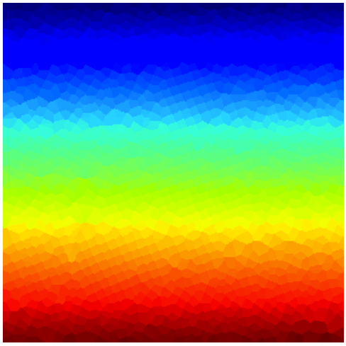
The next step is the computation of the Voronoi diagram. I generated one by brute force: the function scipy.ndimage.distance_transform_edt provides us with an exact euclidean distance transform for any segmentation. Once this transform is computed, I assigned to each pixel the value of the nearest segment.

1
2
L1, L2 = scipy.ndimage.distance_transform_edt(segmentation==0, return_distances=False, return_indices=True)
voronoi = segmentation[L1, L2]

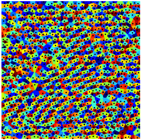
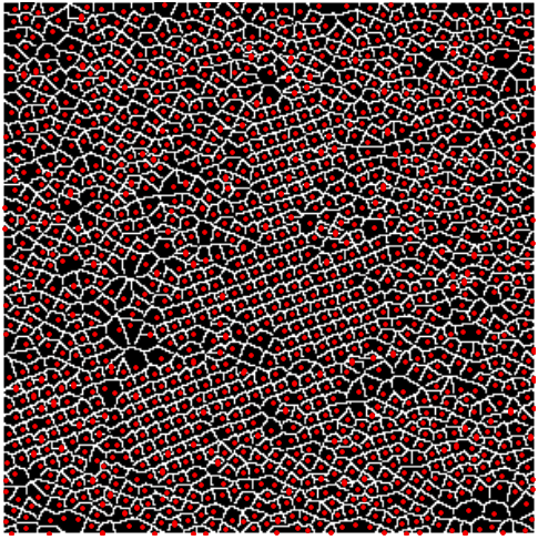
Note that, since there are so many atoms (about 1600), the array stored in voronoi will have those many different colors. A raw visualization of that array will give us little insight on the structural model of the sample (below, left). Instead, we want to reduce the number of “colors”, so that visualization is meaningful. I chose 64 different colors, and used an appropriate colormap for this task (below, center). Another possibility is, of course, to plot the edges of the Voronoi map (not to confuse it with the actual Voronoi diagram!): We can compute these with the simple command

1
2
edges = scipy.misc.imfilter(voronoi, 'find_edges')
edges = (edges  >  0)

In the image below (right) I have included the lattice with the edges of the Voronoi diagram.

But the structural model will not be complete unless we include the information of the chambers of the sample, as well as that of the atoms. The reader will surely have no trouble modifying the steps above to accomplish that task. The combination of the information obtained by merging both Voronoi diagrams accordingly, will yield an accurate model for the sample at hand. More importantly, this procedure can be applied to any micrograph of similar appearance. Note that the quality and resolution of the acquired images will surely enforce different optimal values on thresholds, and fine-tuning of the other variables. But we can expect a decent result nonetheless. Even better outcomes are to be expected when we employ more serious techniques: the segmentation based on thresholding and morphology is weak compared to watershed techniques, or segmentations based on PDEs. Better edge-detection filters are also available.

All the computational tools are amazingly fast and, more importantly, freely available. This was simply unthinkable several years ago.

Generation of figures

One example will suffice. For instance, the commands used to save to png format the last image are given by:

1
2
3
4
5
6
matplotlib.pyplot.figure()
matplotlib.pyplot.axis('off')
matplotlib.pyplot.triplot(triang, 'r.', None)
matplotlib.pyplot.gray()
matplotlib.pyplot.imshow(edges)
matplotlib.pyplot.savefig('/Users/blanco/Desktop/output.png')