The Nonlocal-means Algorithm

The nonlocal-means algorithm [Buades, Coll, Morel] was designed to perform noise reduction on digital images, while preserving the main geometrical configurations, as well as finer structures, details and texture. The algorithm is consistent under the condition that one can find many samples of every image detail within the same image.


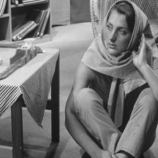
Barbara	Noise added, `std=30`	Denoised image, `h=93`

The algorithm has the following closed form: Given a finite grid \( \Lambda \subset \mathbb{Z}^2 \) of the form \( \Lambda = \Omega \cap \mathbb{Z}^2 \) for some compact set \( \Omega \subset \mathbb{R}^2 \), a signal \( f \in L_2(\Lambda,\mathbb{R}^+) \), and a family of windows \( \{ \mathcal{R}_k \}_{k \in \Lambda} \) satisfying the conditions

\( k \in \mathcal{R}_k \) for all \( k \in \Lambda \).
If \( j \in \mathcal{R}_k \), then \( k \in \mathcal{R}_j \),

the nonlocal-means operator \( \text{NL}_h\colon \ell_2(\Lambda,\mathbb{R}) \to \ell_2(\Lambda,\mathbb{R}) \) with filtering parameter \( h>0 \), is defined by

\begin{equation} \text{NL}_h f(k) = \sum_{j \in \Lambda} \omega_h(j,k) f(j), \end{equation}

where the weights \( { \omega_h(j,k) }_{j,k \in \Lambda} \) are defined by

\begin{equation} \omega_h(j,k) = \frac{ \exp \bigg( -\frac{\left\lVert f(\mathcal{R}_j) - f(\mathcal{R}_k) \right\rVert_{2,a}^2}{h^2} \bigg) }{ \sum_{j \in \Lambda} \exp \bigg( - \frac{\left\lVert f(\mathcal{R}_j) - f(\mathcal{R}_k) \right\rVert_{2,a}^2}{h^2} \bigg)}. \end{equation}

Here, \( f(\mathcal{R}) \) denotes a patch of the image \( f \) supported on the window \( \mathcal{R} \).

Notice that the similarity between patches is nothing but a simple Gaussian weighted Euclidean distance, which accounts for difference of grayscales alone. Efros and Leung prove that this distance is a reliable measure for the comparison of texture patches, and at the same time copes very well with additive white noise; in particular, if \( f \) and \( g \) are respectively the noisy and original images, and \( \sigma^2 \) is the noise variance, then the most similar patches in the noisy image are also expected to be the most similar in the original:

\begin{equation} \mathbb{E} \left\lVert f(\mathcal{R}_j) - f(\mathcal{R}_k) \right\rVert_{2,a}^2 = \left\lVert g(\mathcal{R}_j) - g(\mathcal{R}_k) \right\rVert_{2,a}^2 + 2\sigma^2 . \end{equation}