Binary Images

We can think of a binary image as a True-False map of the form \( f\colon \{ 1, \dotsc, N \} \times \{ 1, \dotsc, M \} \to \{ 0,1 \}. \) These are the simplest images one can imagine, and most of the related image-processing algorithms are trivial to code. For example, take the case of feature recognition:

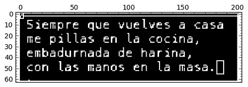
Given the binary image Img below (left) representing a simple text with a few extra features, and any letter of the alphabet, we are able to retrieve all the occurrences of said letter by tracking all the global maxima of a simple correlation (of Img with a suitable image of the required letter as kernel). We have chosen the letter “e” in the following example:

1
2
3
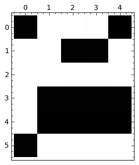
E=Img[8:14,21:26]
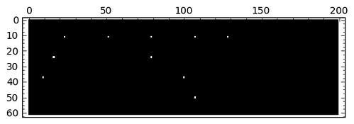
Correlation = scipy.ndimage.correlate(Img,E)
matrix_plot(Correlation == Correlation.max())

A very natural question to ask is, what is a good approximation by binary images to a given gray-scale image \( f\colon \{ 1,\dotsc,N \} \times \{ 1, \dotsc, M \} \to \{ 0, \dotsc, 255 \}? \) Is there any advantage to working with this binary image instead of using the original? Maybe not in general, but for a certain set of simple-enough images, and certain set of image processing procedures, it could turn extremely useful. Let us start by answering first the question of turning grey-scale images into binary:

The half-tone algorithm

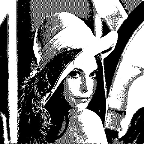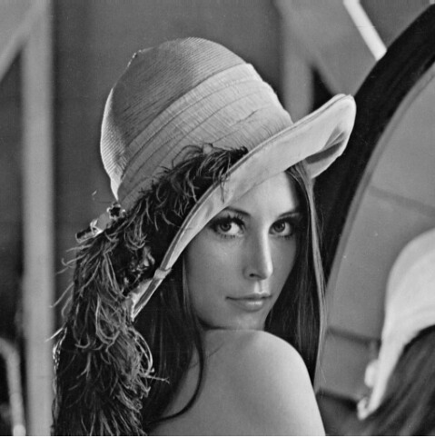
The code below shows an algorithm that performs a simulation of continuous tone images through the use of white and black dots varying in spacing (the closer to each other, the darker; the farther apart, the lighter). It is a good exercise to try and interpret what this code does by yourself, and do a write-up. I helped the process by making the variable names self-explanatory, and dropping small hints. Give it a go!

1
2
3
4
5
6
7
8
9
10
11
12
13
14
15
16
17
18
19
20
21
22
23
24
25
26
27
28
Img = scipy.misc.lena()
GlobalError  = zeros(Img.shape)
ErrorPropagation  = zeros(Img.shape)
HalftonedImg   = zeros(Img.shape)

ColorDistributionKernel   = array([[0,0,7],[2,5,2]])/16.0
threshold=128

for x in range(Img.shape[0]):
    for y in range(Img.shape[1]):
	# We perform some sort of convolution (between what objects?).
	# and store the result in ErrorPropagation
        sum_p=0.0
        for i in range(ColorDistributionKernel.shape[0]):
            for j in range(ColorDistributionKernel.shape[1]):
                xx = minimum(maximum(0,x-i+1),Img.shape[0]-1)
                yy = minimum(maximum(0,y-j+1),Img.shape[1]-1)
                sum_p += ColorDistributionKernel[i,j]*GlobalError[xx,yy]
        ErrorPropagation[x,y]=sum_p
	# How do ErrorPropagation and GlobalError relate to each other?
	# How do we use this to populate the halftoned image?
	# How did we choose the threshold?
        t=Img[x,y]+ErrorPropagation[x,y]
        if t > threshold:
            GlobalError[x,y]=t-2*threshold
            HalftonedImg[x,y]=1
        else:
            GlobalError[x,y]=t