The purpose of this post is to show how histogram equalization improves the quality of digital images: After performing this basic procedure, it will look like new gray scales have been brought up. The truth is that no new gray levels have been introduced: we have simply altered the same gray scales already present in the original, in a way that every value has approximately the same impact. This gives the illusion of darkening bright images, bringing brightness to dark ones, and discovering hidden texture in a priori flat areas.
Let us build the whole project from the ground up, and in the process, illustrate the notion of histogram, as well as the use of many commands for manipulation of arrays and lists in sage.
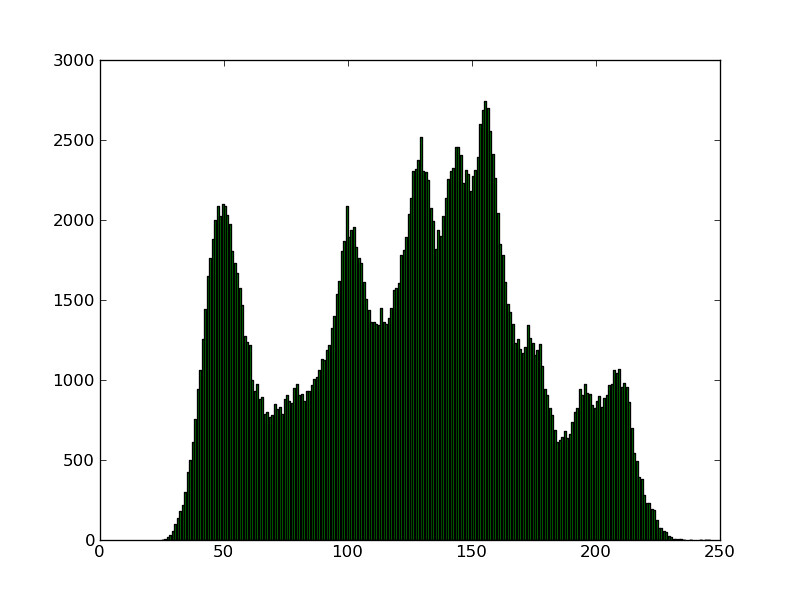
Computing the Histogram
A histogram is nothing but a function that takes as input each of the gray levels present in an image, and offers as output the number of pixels that each of those values share.
1
2
3
4
5
6
7
8
9
10
11
12
13
from numpy import *
import scipy
import matplotlib.pyplot

image = scipy.misc.lena()

Hist = image.flatten().tolist()
grayscales  = uniq(Hist)
frequencies = [Hist.count(x) for x in grayscales]

matplotlib.pyplot.figure()
matplotlib.pyplot.bar(grayscales,frequencies,color='g',edgecolor='k')
matplotlib.pyplot.savefig('/Users/blanco/Desktop/histogram.png')
 |
 |
Of course, there already is a simple (and much faster!) command in sage that will take care of this computation for us: matp.
Histogram Equalization
We alter now the value of each grayscale of the original image, in such a way that the final histogram is as flat as possible, and spreads out over the entire range of the gray levels. We accomplish this by the following procedure:
Assume \( f \colon \{ 1, \dotsc, N\} \times \{ 1, \dotsc, M\} \to \{ 0, \dotsc, 255\} \) is a \( N \times M \) image with 256 gray-scales. We are looking for a function \( \mathcal{E}\colon \{ 0, \dotsc, 255\} \to \{ 0, \dotsc, 255\} \) that performs the histogram equalization: \( g(\boldsymbol{x}) = \mathcal{E} \big( f( \boldsymbol{x}) \big) \).
The way we accomplish it is by:
- Collecting first the histogram of each gray-scale \( k \in \{ 0, \dotsc, 255\}: \) \( H(k) = \# \{ \boldsymbol{x} : f(\boldsymbol{x}) = k \} \)
- Computing the probability of finding a pixel with each gray-scale in the given image: \( p(k) = \frac{1}{NM} H(k). \)
- Computing the cumulative-density function for each gray-scale: \begin{equation} P(k) = \frac{1}{NM} \displaystyle{\sum_{j=0}^k} H(j). \end{equation}
- The histogram equalization \( \mathcal{E} \) simply takes the propability density function for the values in the image \( f \) and multiplies them by the cumulative density function of the values in the image that we seek:
Note that this procedure reduces the number of gray-scales in an image.
1
2
3
4
5
6
7
8
cumsumfreqs = cumsum(frequencies)

histeq = zeros(image.shape)
for index, value in enumerate(grayscales):
    histeq+=cumsumfreqs[index]*(image==value)

histeq /= prod(img.shape)
histeq *= len(grayscales)
 |
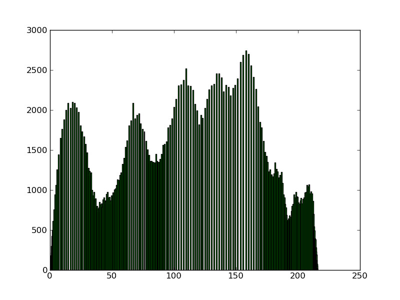 |
As proof of concept, let us compare original with its histogram-equalized version:
|
|
Original | Histogram-equalization |
Note the obvious sharpening of details, albeit the apparent presence of noise where before the image seemed flat. This noise—that we can appreciate for example in the hat or walls—actually reveals a richer texture of the materials photographed. These tectures were not observable directly in the original. Note as well the accentuation of the brightest areas, producing an image with better contrast. I am sure the reader will find some more qualitative improvement in the histogram-equalization version of the image. Working on a set of dark images will reveal even more surprising benefits of this technique.