We have seen a naïve way to perform denoising on images by a simple convolution with Gaussian kernels. In this post I would like to compare that simple method with a more elaborate one: wavelet thresholding. The basic philosophy is based upon the local knowledge that wavelet coefficients offer us: Intuitively, small wavelet coefficients are dominated by noise, while wavelet coefficients with a large absolute value carry more signal information than noise. Being that the case, it is reasonable to obtain a fast denoising of a given image if we perform two basic operations:

• Eliminate in the wavelet representation those elements with small coefficients, and
• Decrease the impact of elements with large coefficients.

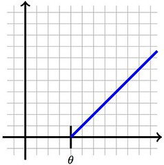
In mathematical terms, all we are doing is thresholding the absolute value of wavelet coefficients by an appropriate function. For example, if we chose to eliminate all coefficients with absolute value less than a given threshold \( \theta \), and keep the rest of the coefficients untouched, we end up with the thresholding function \( \tau_\theta \colon \mathbb{R}^+ \to \mathbb{R} \) given by:

\begin{equation} \tau_\theta (x) = \begin{cases} 0 &\text{if } 0 \leq x\leq \theta \\ x &\text{if } x > \theta\end{cases} \end{equation}

We refer to this function as a hard thresholding. But we might want to decrease the impact of the elements with large coefficients in absolute value—this is what we refer as soft thresholding. A common way to perform this thresholding is by simple imposition of continuity of the function; e.g.:

\begin{equation} \tau_\theta (x) = \begin{cases} 0 &\text{if } 0\leq x\leq \theta \\ x-\theta &\text{if }x > \theta \end{cases} \end{equation}

Other thresholding functions are of course possible, and the reader is encouraged to come up with different examples, and experiment with them.

The wavelet module PyWavelet is easily embedded in sage, and allows us to perform very fast and elegant denoising codes. The following session shows an example: We load the image of Lena as an array of size \( 512 \times 512 \) containing values between 0 and 255. We contaminate the image with white noise \( (\sigma=16.0) \) and perform denoising with this technique. Since \( 512 = 2^9, \) we require all nine levels of the Haar wavelet coefficients of the image.

from numpy import *
import scipy
import pywt

image = scipy.misc.lena().astype(float32)

noiseSigma = 16.0
image += random.normal(0, noiseSigma, size=image.shape)

wavelet = pywt.Wavelet('haar')
levels  = Integer( floor( log2(image.shape[0]) ) )

WaveletCoeffs = pywt.wavedec2( image, wavelet, level=levels)

The object WaveletCoeffs is a tuple with ten entries: the first one is the approximation at the highest level: 9; the second entry is a 3-tuple containing the three different details (horizontal, vertical and diagonal) at the same level. Each consecutive entry is a 3-tuple containing the three different details at lower levels \( (n=8,7,6,5,4,3,2,1) \)

The module pywt has several threshold functions implemented. Let us use the soft thresholding indicated above, with a made-up threshold \( \theta = \sigma \sqrt{2 \log_2(\texttt{image.size})}. \)

In order to apply this threshold to each single wavelet coefficient, we will make use of the powerful tools of functional programming from sage. We need:

• A thresholding function. We use the ones provided by the pywt package: pywt.thresholding.soft, and in particular its lambda expression:

lambda x: pywt.thresholding.soft(x, threshold)

• Python’s built-in function map(func, seq1, seq2, ...)
• The tuple of objects over which we need to apply the thresholding: In this case, the set of wavelet coefficients WaveletCoeffs computed above.

Once computed the new coefficients, we use pywt.waverec2 to obtain the corresponding reconstruction:

threshold = noiseSigma*sqrt(2*log2(image.size))
NewWaveletCoeffs = map (lambda x: pywt.thresholding.soft(x,threshold), WaveletCoeffs)
NewImage = pywt.waverec2( NewWaveletCoeffs, wavelet)

original + noise	denoised (`haar`)

Denoising is good, but the overall visual quality of the resulting image is very poor: there are many artifacts, due mainly to the blocky nature of the Haar wavelet. Also, the choice of threshold is artificial: it has a priori no relationship with the structure of the image. Let’s put a temporary solution to this problem by using a smoother wavelet, while keeping the same threshold. To avoid excessive typing, we will wrap the code above into a neat function with variables being the image to be treated, the standard deviation of the noise added, and the name of the wavelet employed:

def denoise(data,wavelet,noiseSigma):
    levels = Integer(floor(log2(data.shape[0])))
    WC = pywt.wavedec2(data,wavelet,level=levels)
    threshold=noiseSigma*sqrt(2*log2(data.size))
    NWC = map(lambda x: pywt.thresholding.soft(x,threshold), WC)
    return pywt.waverec2( NWC, wavelet)

We can now perform the same operation with different wavelets.  The following script creates a python dictionary that assigns, to each wavelet, the corresponding denoised version of the corrupted Lena image.

Denoised={}
for wlt in pywt.wavelist():
    Denoised[wlt] = denoise( data=image, wavelet=wlt, noiseSigma=16.0)

The  four images below are the respective denoising by soft thresholding of wavelet coefficients on the same image with the same level of noise \( (\sigma = 16.0), \) for the symlet sym15, the Daubechies wavelet db6, the biorthogonal wavelet bior2.8, and the coiflet coif2. Note that, except in the case of the denoising by biorthogonal wavelet, all of the others present clear artifacts:

denoised (`sym15`)	denoised (`db6`)
denoised (`bior2.8`)	denoised (`coif2`)