The unit sphere in any \( d \)–dimensional space \( \mathbb{R}^d \) is defined to be the set \( \mathbb{S}_{d-1} = \big\{ (x_1,x_2,\dotsc,x_d) \in \mathbb{R}^d : \sum_{k=1}^d x_k^2=1 \big\}. \)  The 1-dimensional sphere is, of course, the circle, that we can parametrize by angles:

\begin{equation} \varphi \colon [0,2\pi) \in \theta \mapsto e^{i\theta} = \cos \theta + i \sin \theta \equiv (\cos \theta, \sin \theta) \in \mathbb{S}_1 \end{equation}

While understanding the definition of homeomorphism, we worked on such a map from a disk \( D_2 \) to a square \( \square_2. \)  In this section we are going to use this idea to establish a homeomorphism between the 2-dimensional sphere \( \mathbb{S}_2 \subset \mathbb{R}^3 \), and the quotient space formed by a proper identification of points in the border of a square \( \square_2 \subset \mathbb{R}^2. \)  The construction goes as follows:

1. Scale the unit sphere by a half, and shift it vertically up by half unit, so the center is at \( (0,0,\frac{1}{2}). \)
2. The plane \( { x_3=0} \) intersects this sphere at the origin.  We identify this point with the center of the disk \( D_2. \)
3. For each \( 0 \leq \lambda < 1, \) the horizontal plane \( {x_3=\lambda} \) intersects this sphere in the circle \( \big\{ (x_1,x_2,\lambda) \in \mathbb{R}^3 : x_1^2 + x_2^2 + (\lambda - \frac{1}{2})^2 = \frac{1}{4} \big\}: \) the center is at \( (0,0,\lambda), \) and the radius is \( \sqrt{\frac{1}{4}-(\lambda-\frac{1}{2})^2}. \)
   We consider a map that scales this circle to that of radius \( \lambda, \) and “places it” on the unit disk \( D_2 \) in a natural way.  So far, the map so constructed is injective, onto and continuous.

4. The issue now is what to do with the last non-void intersection of the sphere with horizontal planes.  This happens at the horizontal plane \( { x_3 = 1}, \) and the result is the only point \( (0,0,1). \)  We overcome this situation by mapping the whole point into the last circle in \( D_2 \), and identifying the whole circle.  We accomplish this by creating the equivalence relation \( (x_1,x_2) \sim (y_1,y_2) \) defined by the following rules:

   1. \( x_1=y_1 \) and \( x_2=y_2, \) or
   2. \( x_1^2+x_2^2=y_1^2+y_2^2=1. \)

We have thus created a homeomorphism \( \varphi_1 \colon \mathbb{S}_2 \to D_2. \)  Compose this with an homeomorphism \( \varphi \colon D_2 \to \square_2, \) and notice that the equivalence relation defined above turns into the equivalence relation \( (x_1,x_2) \sim (y_1,y_2) \) defined by the following rules:

1. \( x_1=y_1 \) and \( x_2=y_2 \), or
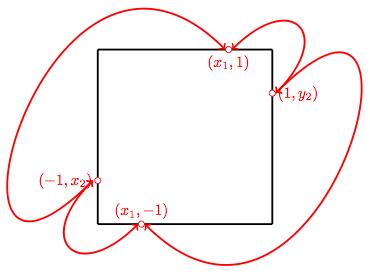
2. \( \mathop{\text{max}}\big(\lvert x_1\rvert, \lvert x_2\rvert \big) = \mathop{\text{max}}\big( \lvert y_1\rvert, \lvert y_2\rvert \big) = 1. \)

Graphically, we represent this set with the diagram below: