Consider in the sphere \( \mathbb{S}_2 \subset \mathbb{R}^3, \) the relation induced by identification of antipodal points; that is, given \( z_1, z_2 \in \mathbb{S}_2 \), set \( z_1 \sim z_2 \) if and only \( z_1 = \pm z_1. \) The corresponding quotient space \( \mathbb{P} = \big( \mathbb{S}_2 / \sim \big) \) is what we call real projective space.

Since we are interested in the topological properties of this space, we actually define a real projective space to be any homeomorphic set to \( \mathbb{P}. \)  Among those, we are interested in one that can be realized from a square, by identification of its sides (in a similar manner as we did with the torus).  We proceed as follows:

Assume that we start from the unit sphere \( \{ (x_1,x_2,x_3) \in \mathbb{R}^3 : x_1^2+x_2^2+x_3^2=1 \} \), and note that the upper hemisphere \( H=\{ (x_1,x_2,x_3) \in \mathbb{R}^3 : x_1^2+x_2^2+x_3^2=1, x_3 \geq 0 \} \) contains at least one of each pair of antipodal points.  If both antipodal points occur in \( H \), they will necessarily lie over the circle \( \{ (x_1, x_2, 0) \in \mathbb{R}^3 : x_1^2+x_2^2=1 \}. \)  The hemisphere \( H \) is obviously homeomorphic to a disk (by a simple vertical projection onto the plane \( \{x_3=0 \}, \) for example).  And the disk is homeomorphic to a square, so we may use a composition of both to realize a homomorphism from \( H \) to \( \square_2. \)

Define in \( H \) an equivalence relation that identifies two antipodal points on the border, and notice that the homeomorphism just computed takes that identification to the following: Given \( (x_1,x_2), (y_1,y_2) \in \square_2 \), it is \( (x_1,x_2) \sim (y_,y_2) \) if

• \( x_1=y_1 \) and \( x_2=y_2 \), or
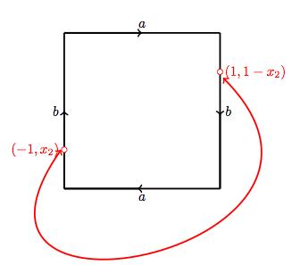
• \( x_1y_1 = -1 \) and  \( x_2=1-y_2 \), or
• \( x_2y_2=-1 \) and \( x_1=1-y_1 \).

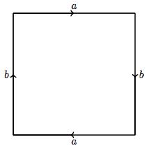
A diagram representing the quotient space \( \big( \square_2 / \sim \big) \) is presented below:

The punch-line is, of course, to construct a homeomorphism from the real projective plane \( \mathbb{P} \) as defined above, to the quotient space \( \big( \square_2 / \sim \big). \) The reader should not have much trouble to give an analytic expression of such a map following the steps above.