A Hausdorff space \( X \) is said to be a \( d \)–dimensional manifold if, for each \( p \in X \) there exists an open neighborhood of \( p \) which is homeomorphic to the unit \( d \)–dimensional Euclidean ball \( D_d = \big\{ (x_1,\dotsc, x_d) \in \mathbb{R}^d : \sum_{k=1}^d x_k^2 < 1 \big\}. \) We also refer to them as \( d \)–manifolds and, in the case \( d=2 \), by the name of surfaces.
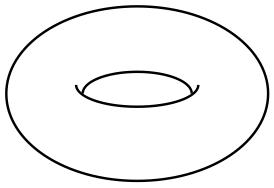
The sphere \( \mathbb{S}_2 \), the torus \( \mathbb{T} \) and the real projective plane \( \mathbb{P} \) are all well-defined surfaces, as the reader will surely have no trouble proving. The three share several topological properties: they are all connected and compact. The sphere and the torus differ, nonetheless, in the number of “holes” that they present (we will make this notion more precise later on). The real projective plane, unlike the other two, is non-orientable (we will work on this idea later too). These three are fundamentally different surfaces. A natural question then arises: What are all the possible compact-connected surfaces?
But “gluing” together two or more surfaces, we can construct new examples. Let us give a formal definition of this intuitive “gluing” of surfaces, and explore its properties: Let \( S \) and \( S’ \) be two surfaces, and let \( D \subset S \), \( D’ \subset S’ \) two sets homeomorphic to a closed disk \( \overline{D_2} \). The borders of both sets—\( \delta D \) and \( \delta D’ \) respectively—are homeomorphic to a circle, and thus we can find a homeomorphism \( \varphi \colon \delta D \to \delta D’. \) We then define the connected sum of the surfaces \( S \) and \( S’, \) to be the quotient set obtained on the union
after identification of the borders \( \delta D \) and \( \delta D’ \) via the previous homeomorphism \( \varphi. \) This is: If \( p,q\in\big(S\setminus\overset{\circ}{D}\big)\cup\big(S’\setminus\overset{\circ}{D’}\big), \) then \( p \sim q \) provided
- \( p = q \), or
- \( p \in \delta D, q \in \delta D’, \) and \( q=\varphi(p), \) or
- \( p \in \delta D’, q \in \delta D, \) and \( p = \varphi(q). \)
We denote \( S \mathop{\#} S’=\bigg(\big(S\setminus\overset{\circ}{D}\big)\cup\big(S’\setminus\overset{\circ}{D’}\big)/\sim\bigg) \).
Let us show with an example the connected sum of two torii:
 |
|
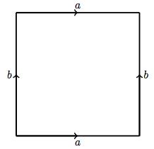
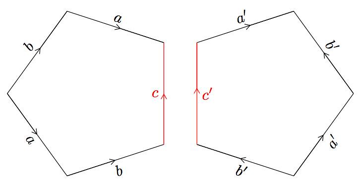
The connected sum of two tori start with the two surfaces next to each other. The diagram below represents the corresponding homeomorphic squares, with the edges identified according to the proper equivalence relation. |
 |
|
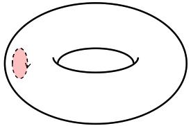
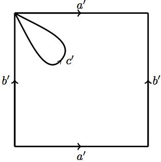
| In the second step, we remove from each torus a set homeomorphic to a closed disk. The borders of each disk are homeomorphic, and we consider such an homeomorphism for the gluing of the surfaces in the next step. We indicate this in the diagram by specifying a direction in both borders. |  |
 |
 |
 |
|
 |
||
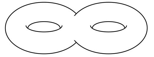 |
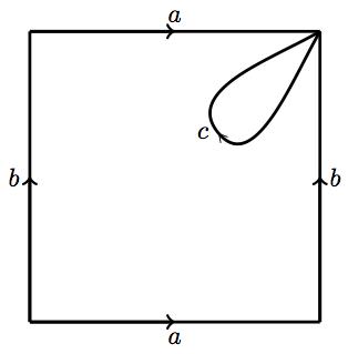
The result is a torus with two holes (we prefer to use the word genus to refer to them). The diagram shows how to obtain the corresponding polygon, after identification of the paths \( c \) and \( c'. \) It is not hard to prove that the polygon with identified sides as shown is indeed homeomorphic to the genus-two torus above, via the homeomorphisms constructed in previous pages. |
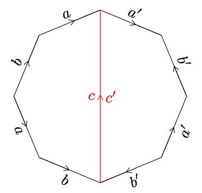 |
The reader will notice that all of the vertices of this polygon are actually the same vertex! Pick any vertex, say \( P \) between edges \( a \) and \( a’. \) Since it is at the end of (directed) edge \( a, \) this vertex \( P \) is also the same as the one between edges \( a \) and \( b. \) As it is now at the beginning of edge \( b, \) it must be also \( P \) between the edges \( b \) and \( a. \) This proves that \( P \) is also at the beginning of edge \( a. \) We can continue in this fashion to realize that, indeed, we can safely label \( P \) all of the vertices of this polygon.