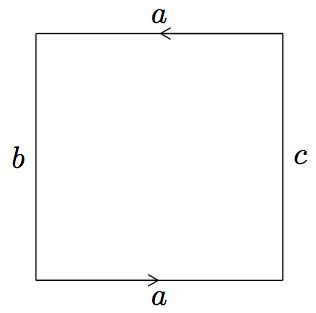
Consider a long and narrow strip of paper, in which we glue the two narrower edges together after performing a half-twist of the strip, hence forming a funny-looking loop. Topologically, this is equivalent to identifying two parallel edges of a square in the proper way. Therefore, we can see the Möbius band as the quotient space of \( \square_2 \) with the following equivalence relation: Given \( (x_1,x_2), (y_1,y_2) \in \square_2, \) we write \( (x_1,x_2) \sim (y_1,y_2) \) if
- \( x_1=y_1 \) and \( x_2=y_2, \) or
- \( x_2 y_2 = -1 \) and \( x_1 = 1-y_1. \)
 |
 |
In a similar fashion, we construct a new surface by identification of two parallel edges of a square to form a cylinder, and a posterior identification of the remaining two edges (which turned into two circles after the first identification). The second identification will be performed after a “half-twist” (which unfortunately can only be realized in a fourth dimension!). The equivalence relation in the square \( \square_2 \) is as follows: Given \( (x_1,x_2), (y_1,y_2) \in \square_2, \) we define \( (x_1,x_2) \sim (y_1,y_2) \) provided one of the following conditions are satisfied:
- \( x_1=y_1 \) and \( x_2=y_2, \) or
- \( x_1 y_1 = -1 \) and \( x_2 = y_2 \), or
- \( x_2 y_2 = -1 \) and \( x_1 = 1-y_1. \)
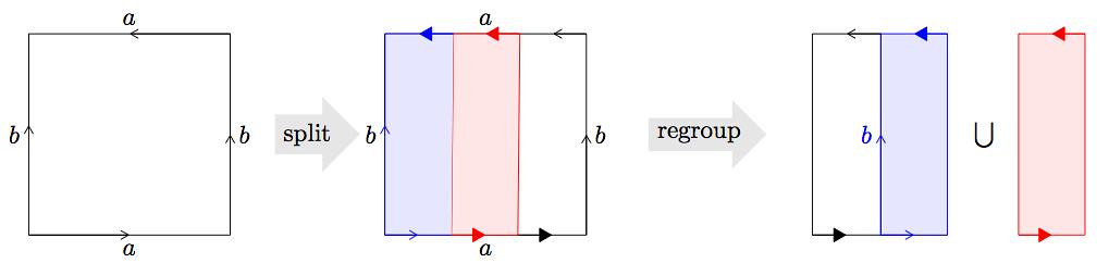
A diagram representing this quotient space—which we denote \( \mathbb{K} \) and call Klein bottle—is shown below, together with an interesting way to split and recover the space: Notice how by cutting three stripes in the manner shown, and adjoining two of the stripes through the proper edge, we can see the Klein’s bottle as the union of two Möbius bands.
Miscellaneous
All the images included in this presentation are generated with the aid of the package tikz in \( \LaTeX \). The code that created the Möbius strip above, for example, is given by
1
2
3
4
5
6
7
8
9
10
11
12
13
14
15
16
17
18
19
\documentclass{amsart}
\usepackage{tikz}
\usetikzlibrary{calc}
\begin{document}
\begin{tikzpicture}
\coordinate (a) at (0cm,0cm);
\coordinate (b) at (1cm,0cm);
\coordinate (c) at (60:1cm);
\coordinate (ab1) at ($ (a)!.25!(b) $);
\coordinate (ab2) at ($ (a)!.75!(b) $);
\coordinate (bc1) at ($ (b)!.25!(c) $);
\coordinate (bc2) at ($ (b)!.75!(c) $);
\coordinate (ac1) at ($ (a)!.25!(c) $);
\coordinate (ac2) at ($ (a)!.75!(c) $);
\draw[fill=red!60!black,thick,rounded corners=2pt] (ab1) -- (bc2) [rounded corners=1pt] --(ac2) -- (ac1) [rounded corners=2pt] --cycle;
\draw[fill=red!80!black,thick] (bc1) [rounded corners=2pt] --(bc2) [rounded corners=1pt]-- (ac2) [rounded corners=2pt]-- (ab2) [rounded corners=1pt] --cycle;
\draw[fill=red,thick] (ab1) [rounded corners=2pt] -- (ab2) [rounded corners=1pt] -- (bc1) -- (ac1) [rounded corners=2pt] -- cycle;
\end{tikzpicture}
\end{document}