Toying with basic fractals
I will skip all the mathematical theory behind Fractals (dimensions, measures, etc) to focus directly into the description and implementation of some of the most basic examples. In this post, I will cover the ideas behind three classical techniques:
- Iterated function systems
- Membership tests
- Lindenmayer systems
Fractals from Iterated Function Systems
We start from an affine transformation \( f\colon \mathbb{R}^2 \to \mathbb{R}^2, \) described as a shift with direction \( \boldsymbol{b}=(b_1,b_2) \) of a linear transformation \( A=\big(\begin{smallmatrix}a_{11}&a_{12}\\ a_{21}&a_{22}\end{smallmatrix}\big)\):
Given a single point \( \boldsymbol{x} \in \mathbb{R}, \) and an affine transformation as above, consider the sequence formed by applying the same transformation on successive outputs:
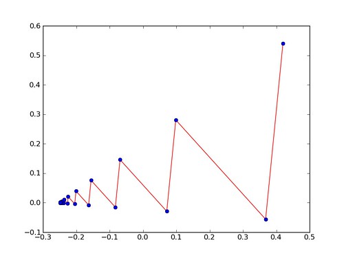
For example, for the point \( \boldsymbol{x}=(0.42,0.54) \) and the affine transformation given by \( A=\tfrac{1}{10} \big( \begin{smallmatrix} 6&4\\ 4&-6\end{smallmatrix}\big), \) and \( \boldsymbol{b}=(-0.1,0.1), \) the graph below shows the behavior of the sequence. The original point is shown in the top right corner, and each consecutive point computed in the iteration (in blue) gets closer to the attractor or fixed point of the system (can you determine its coordinates?). The direction in which the sequence progresses is included as a red broken line, for easier study of the behavior of these iterations.
1
2
3
4
5
6
7
8
9
10
11
12
pt=[0.42, 0.54]
A=[pt]

for k in range(20):
    pt = [ 0.4*pt[0] + 0.6*pt[1] - 0.1, 0.6*pt[0] - 0.4*pt[1] + 0.1 ]
    A.append(pt)

import matplotlibs.pyplot
matplotlib.pyplot.figure()
matplotlib.pyplot.plot(*zip(*A), color='r')
matplotlib.pyplot.plot(*zip(*A), marker='o', ls='', color='b')
matplotlib.pyplot.savefigure('/Users/blanco/Desktop/sequence.png')
Based on this simple construction, Michael Barnsley proposed the following so-called Chaos game: choose a point \( \boldsymbol{x} \in \mathbb{R} \) in the plane, and several different affine transformations \( f_1, f_2, \dotsc, f_n. \) Assign to each transformation a different probability \( P(f_k)=p_k, \) for \( k=1,2,\dotsc,n, \) so that \( p_1+p_2+\dotsb+p_n=1. \) Allow the point to be transformed by a random choice of \( f_k, \) so that the frequency of choice is governed by their respective probabilities. The following example indicates a possible outcome:
Set \( \boldsymbol{x}=(0,0), \) and consider the four affine maps below, with their corresponding probabilities:
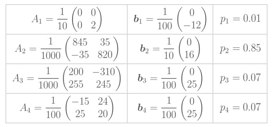
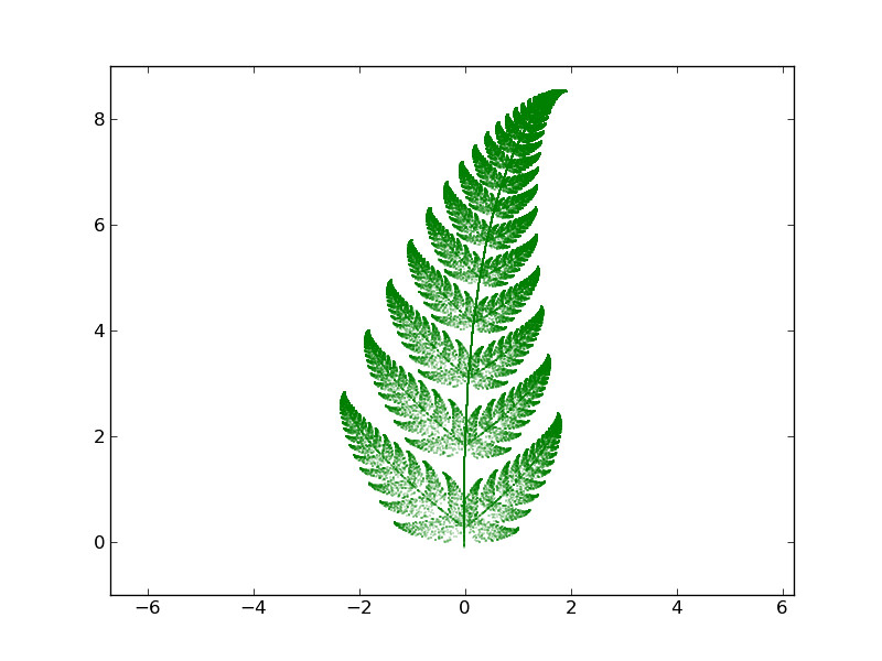
What we see is a large set of points (100,000) that are close to a fractal fern: the attractor (or the set of fixed points) of the system of iterations given above.
A nice coding exercise is the creation of a function that offers as outputs the graphs of the clouds of points obtained: Collect the data from the IFS in a single matrix of size \( 7\times n, \) and use it as input of a script that, in a similar way to the toy example above, plots a large number of iterations of this system.
Membership tests
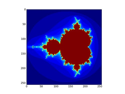
In membership tests, each point of a lattice of the plane is tested for membership in a given fractal set. This membership test may be defined in many different ways. The typical example is given by the Mandelbrot set: We identify each point \( \boldsymbol{x}=(x_1,x_2) \in \mathbb{R}^2 \) in the plane with a complex number \( \boldsymbol{c}=x_1+i x_2 \in \mathbb{C} \) in the usual way, and with the quadratic polynomial \( P_{\boldsymbol{c}}\colon\mathbb{C}\to\mathbb{C} \) given by \( P_{\boldsymbol{c}}(z) = z^2+\boldsymbol{c}. \) We say that the point \( \boldsymbol{x} \) belongs in the Mandelbrot set provided that the sequence of iterations \( \big( P_{\boldsymbol{c}} \circ P_{\boldsymbol{c}} \circ \stackrel{(n)}{\dotsb} \circ P_{\boldsymbol{c}} \big) (\boldsymbol{0}) \) does not tend to infinity. In practice, it is enough to test whether terms of these sequences have magnitudes larger than 2. A simple script that approximates this set on a grid of size \( 256 \times 256 \) by testing after thirty iterations is shown below:
1
2
3
4
5
6
7
8
9
10
11
12
13
14
15
16
17
18
19
20
21
22
23
24
25
from numpy import *

length,width,iterations = 256,256,30

# Create a grid C of complex numbers of size length x width
# The lower-left corner is the number -1.4-2i
# The upper-right corner is the number 1.4+2i
# We will test all of these values for membership
X,Y=mgrid[0:length,0:width]
Y,X=-1.4+2.8*Y/(width-1), -2+2.8*X/(length-1)
Z=X+i*Y
C=X+i*Y

# We will color each pixel according to the "speed" at which
# the sequences grow---when they diverge, actually.
mandelbrot = iterations + zeros(C.shape)

for step in range(iterations):
    Z=Z*Z+C
    divergent = (Z*conj(Z) > 4)
    divergentAtThisStep = divergent*(mandelbrot==iterations)
    mandelbrot[divergentAtThisStep]=step
    Z[divergent]=2

mandelbrot.transpose()
Lindenmayer systems
Start with a simple chain of commands, coded by symbols: for example: “Go forward one unit (F), turn left 60º (X), go forward one unit (F), turn right 120º (Y), go forward one unit (F), turn left 60º (X), go forward one unit (F)”—coded as FXFYFXF. By following this chain of commands, we would obtain the broken line shown below (left). We also have a set of rules that change some of the symbols. In this case, we will require one rule alone: turn each occurrence of F into the string FXFYFXF. Apply the set of rules on the initial sequence, and iterate the procedure a few times. For example, after two iterations, we have the string
A suitable interpreter that follows each command appropriately, will produce the broken line below (right).
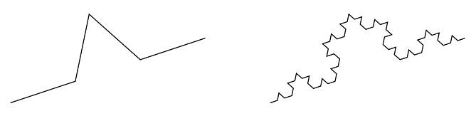
In this case, the fractal is the broken line that results after taking this iteration to the limit: it can be proved that it has an infinite length, and it has many other interesting properties.
The \( \LaTeX \) package tikz offers us a very simple syntax to produce approximations to this so-called Koch snowflake, as well as some other well-known fractals. By including the tikz library decorations.fractals, the two curves mentioned above could be obtained as follows:
1
2
3
4
5
6
\begin{center}
  \begin{tikzpicture}[decoration=Koch snowflake]
    \draw decorate{ (0,0) -- (3,1) };
    \draw decorate{ decorate{ decorate{ (4,0) -- (7,1) } } };
  \end{tikzpicture}
\end{center}
We can obtain decorative fractal-based image generated with tikz, by issuing very simple commands:
1
2
3
4
5
6
\begin{tikzpicture}[decoration=Koch snowflake,scale=2]
  \draw decorate{ decorate{ decorate{ decorate{ (0,0) --
          (4,0) -- (4,4) -- (0,4) -- cycle } } } };
  \draw decorate{ decorate{ decorate{ decorate{ (2,1.5) --
          (2.5,2) -- (2,2.5) -- (1.5,2) -- cycle } } } };
\end{tikzpicture}